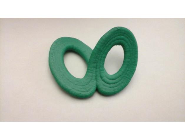
Lorenz Attractor

thingiverse

A 3D rendering of the Lorenz attractor emerges by traversing the parametric path multiple times around each loop and thickening it to form a solid shape. The design begins in Sage, where the program is exported as an X3D file. This resulting file is then edited in Blender to remove any artifacts left behind by Sage, such as a cube of lines surrounding the figure. Next, the X3D file is exported again, this time as an STL file, which is imported into Cura. Here, the figure is scaled up because graph units in Sage are converted to millimeters in Cura. The figure is then situated on the print platform, and the STL file is exported once more to form the STL thing file. The Sage code used to generate this 3D model is as follows: x, y, z, t = var('x, y, z, t') sigma = 10 rho = 28 beta = 8 / 3 lorenz = [sigma * (y - x), x * (rho - z) - y, x * y - beta * z] s = desolve_system_rk4(lorenz, [x, y, z], ics=[0, 0, 1, 21.5], ivar=t, end_points=10, step=0.05) sol = [[q[1], q[2], q[3]] for q in s] p = Graphics() p += line3d(sol, thickness=27, corner_cutoff=0.05) p.show() As Sage is based on Python, be sure to check the line breaks carefully. This code utilizes the built-in Runge-Kutta version of the desolve() method. The outcome is a list of points providing a parametric representation of the solution curve, which is plotted here using line3d() with "thickness" set high enough to make the figure appear solid.